Convex Set
Definition a line connecting to line in the sets is constrained in the set. The simple terms is we can connect any two points inside the set with a line. In condition that the line which connects the two points is inside the sets.
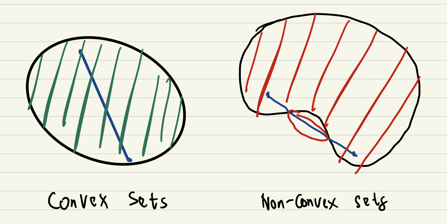
Examples of Convex Sets:
Linear Subspace\(Ax =b\)Half-space, Hyperplane, Polytope\(Ax \leq{b}\)Elipsoids\(x^TPx \leq 1, P \gt 0\)Cones\(\| x_{2:n}\|_2 \leq x_1\)
Convex Function
\(\text{A function} \, f(x) : \mathbb{R^n} \rightarrow \mathbb{R} \, \text{whose epigraph is a convex set.}\)
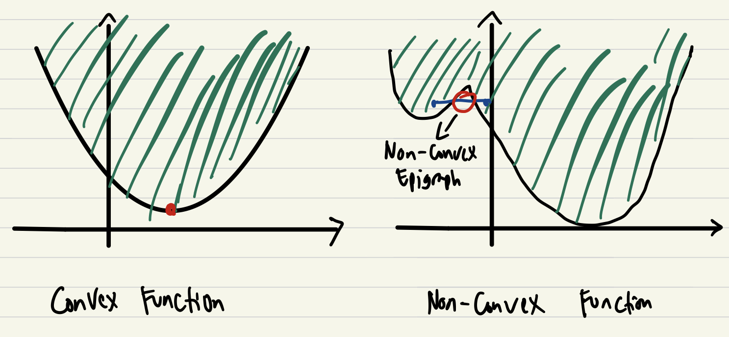
But what is epigraph? Everything above the function lines is called epigraph (dark green hatched area in the figure above).
Examples of Convex Function:
Linear\(f(x) = c^Tx\)Quadratic\(f(x) = \frac{1}{2}x^TQx + q^Tx, Q \gt{0}\)Norms (Any Norms)\(\lvert x \rvert\)
Convex Optimization Problem
Generally, solving a convex optimization problem is minimizing a convex function over a convex sets.
Examples of Convex Optimization Problem:
Linear Program (LP)\(\begin{aligned} \text{linear cost function} \, f(x) \, \text{and} \, \text{linear constraints} \, c(x) \end{aligned}\)Quadratic Program (QP)\(\begin{aligned} \text{quadratic cost function} \, f(x) \, \text{and} \, \text{linear constraints} \, c(x) \end{aligned}\)Quadratically Constrained QP (QCQP)\(\begin{aligned} \text{quadratic cost function} \, f(x) \, \text{and} \, \text{elipsoid constraints} \, c(x) \end{aligned}\)Second Order Cone Program (SOCP)\(\begin{aligned} \text{linear cost function} \, f(x) \, \text{and} \, \text{conic constraints} \, c(x) \end{aligned}\)
In the Convex Optimization, there is no spurious local optima solution. Technically, if we manage to find the local optima Karush–Kuhn–Tucker (KKT) condition it will be our global solution.
Newton’s Method can work really well and converge really fast with 5~10 iterations (able to bound solution for the real-time control).