Model Predictive Path Integral Control (MPPI) (ICRA 2016, IEEE T-RO 2018)
The path integral control framework is a way to solve an optimal control problem by generating stochastic samples of the trajectories. In path integral control, the value function of the optimal control problem is transformed into a path integral, which is an expectation over all possible trajectories. The path integral allows the stochastic optimal control problem to be solved with a Monte Carlo approximation.
In previous works before MPPI, there were various algorithms in the path integral control setting (e.g., model predictive control, policy improvement with Path Integrals, and Iterative Feedback). However, those algorithms are limited in their behavior and do not consider the full Nonlinearity of Dynamics.
Another efficient and better approach is to use a GPU to exploit the parallel nature of sampling so that thousands of samples of trajectories from nonlinear dynamics can be sampled without a problem. Nevertheless, the expectation is taken with respect to the uncontrolled dynamics (u=0), which means that the probability of sampling a low-cost trajectory is technically very low.
In the initial version of MPPI (ICRA 2016) MPPI only worked with the control affine dynamics and didn't work with the arbitrary nonlinear dynamics, therefore in the next version of MPPI (T-RO 2018) MPPI that works with any nonlinear dynamics is presented
Core Ideas of MPPI (from the Learning to Control 2021 Tutorial):
- Based on
Model Predictive Control (MPC)
- Simulate into the future
(running thousands of rollouts)
- From the rollout results, which
have randomly different inputs (we can understand whether it is good or bad)
- The
best input will be the weighted sum of inputs
- The rollout
has low cost → larger weights
Update inputs and repeat again
The MPPI Algorithm
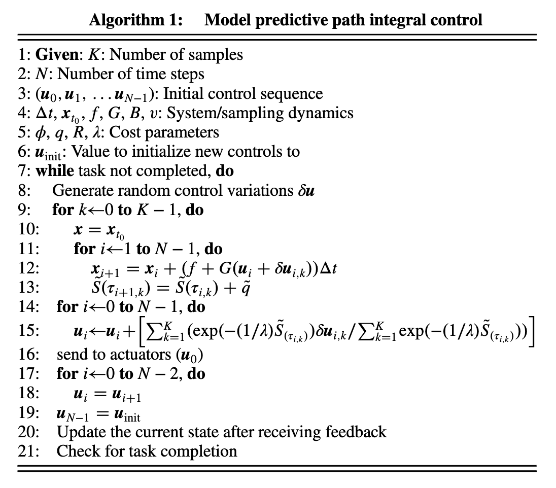
Explanation of the Algorithm
Define your horizon steps and the number of trajectory samples (line 1 and 2)
Initialize control sequence (line 3)
while task not completed, do:
Generate random pertubationsδu
for Monte Carlo rollouts k=1...K do:
Start in current statexk,0=x(t0)
for MPC horizon steps n=0..N-1 do:
Inputuk,n=un+δuk,n
Next statexk,n+1=model(xk,n,uk,n)
Rollout costSk=Sk+stagecostqk,n
end
end
for n=0 .. N-1 do:
un=un+reward weighted perturbations
end
Apply first inputu0
Get system feedback
Check if the task completed
end
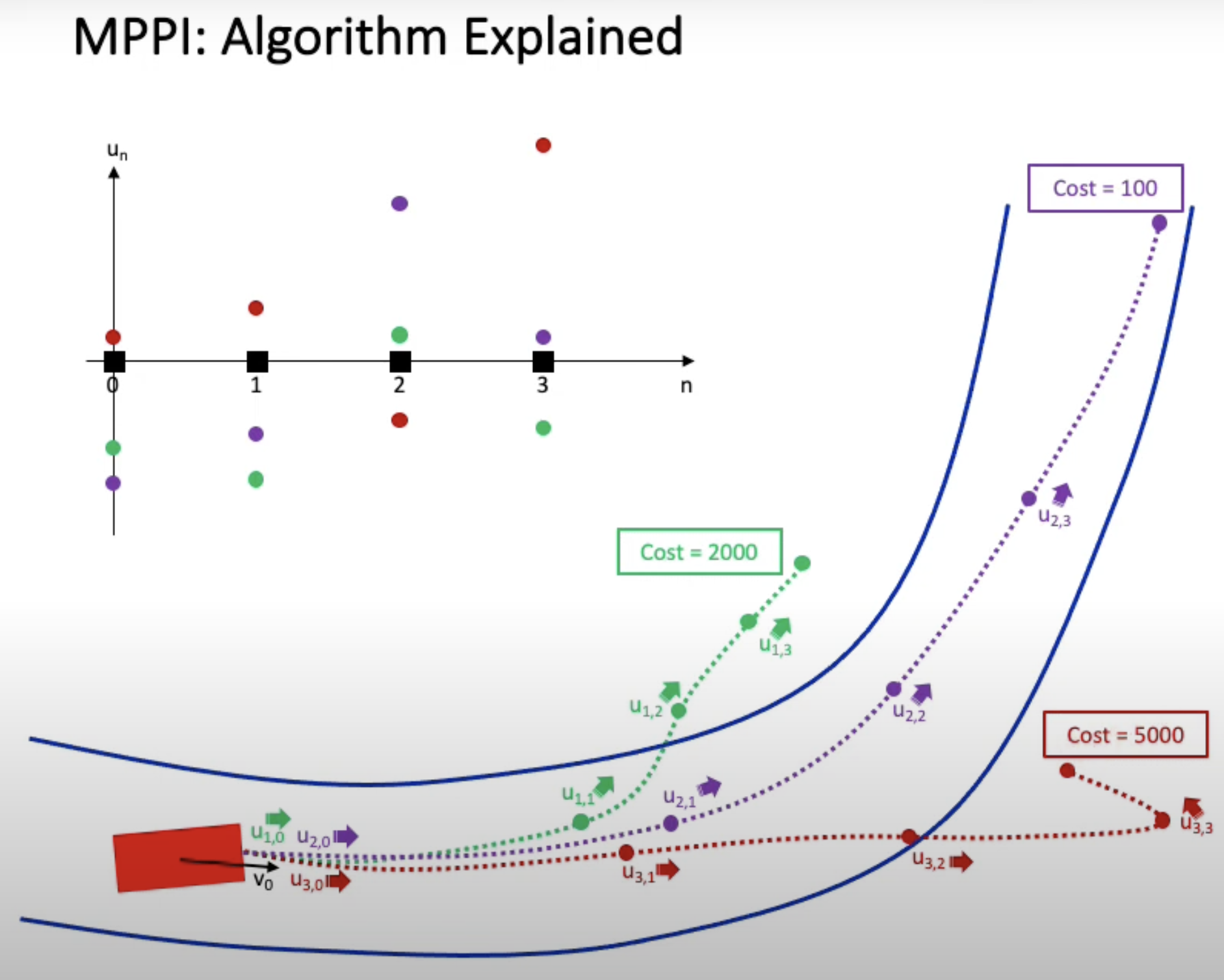
Let’s say we are going to define the MPC with N=5 horizon steps (line 2)
With K=4 samples of random disturbance vectors (line 1)
δuk∈R5
Then, we are going to have 4 sampled rollouts (line 8) δu1,δu2,δu3,δu4
In rollout k, apply the disturbed input vector within the horizon length (line 15)
u+δuk∈R5,u is the nominal input
Updating the nominal input with reward weighted perturbations u=u+∑wk∑wkδuk
Where the weights are wk=e−λ1Sk
Sk:cost of trajectory kλ:constant parameter
References:
- Learning to Control 2021 Tutorial
- G. Williams, P. Drews, B. Goldfain, J. M. Rehg, and E. A. Theodorou, “Aggressive driving with model predictive path integral control,” 2016 IEEE International Conference on Robotics and Automation (ICRA)
- Model Predictive Path Integral Control: From Theory to Parallel Computation Grady Williams, Andrew Aldrich, and Evangelos A. Theodorou, Journal of Guidance, Control, and Dynamics 2017
- Williams, Grady, et al. “Information-theoretic model predictive control: Theory and applications to autonomous driving.” IEEE Transactions on Robotics 34.6 (2018): 1603-1622.